Part 1: Architectural and Algorithmic Optimisations in LLM Inference

What 20+ Papers and Open-Source Projects Taught Me About Cracking LLM Inference

If you’re developing AI solutions and hosting foundation models built around large language models (LLMs), you should think about the cost of serving them. However, money is not the only consideration; believe me, if you cannot fix difficulties with model performance, even if you have a large budget, serving LLMs will suffer. This paper discusses the challenges of changing your LLM inference from a money drain to a high-throughput engine.

Challenges in LLM Serving

LLMs are amazing, but their characteristics make them hard to serve. An LLM inference has two phases:

1. Prefilling:  When you input the prompt (context, conversation history, question, etc.), the model processes all the tokens simultaneously.
2. Decoding: After the initial prompt, the model generates one token at a time, and the new token depends on the previous ones.

For easy imagination, prefilling is equivalent to setting up the board for a chess game (takes time), while decoding is similar to playing move by move after setup (each move is fast).

Unfortunately, LLMs serving is not like eating a piece of cake; some problems must be considered:

Sparsity

In neural networks, specifically FFN, many neural values are zero, skipping these zero neural values and focusing only on non-zero elements will save us time in operation.

Several neural in a LLM is zero value, this causes much zero value in matrix multiple. Image source

Memory Bandwidth Limits and Memory Bound

Moving data on/off the GPU often consumes more time than computation. Plus, the size of a big model, such as Chatgpt, which, by myth, is said to contain a trillion parameters, could not fit in one single GPU.

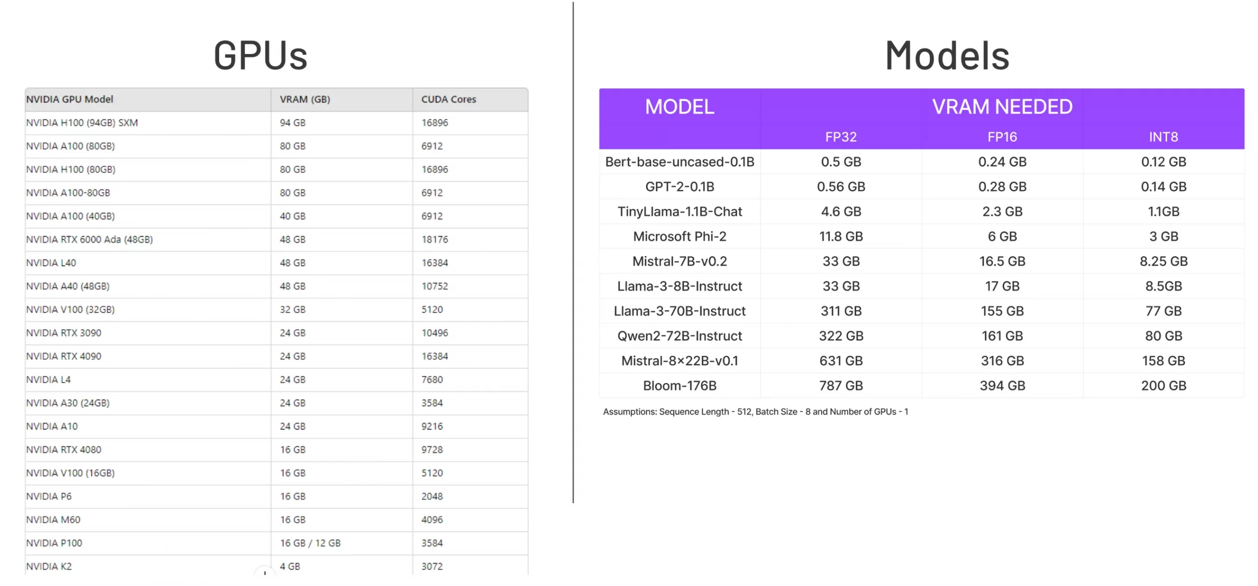
Comparison to the state-of-the-art models to GPUs memory. Image source: Chatgpt

Poor Scheduling — First come, first served

LLMs often serve multiple requests at a time. This scenario draws a situation where short requests, such as asking about the weather, time, and short answers, must wait to process the long ones. Then, the average reply time is almost entirely due to waiting time, not the computation time.

You ‘re faster but you must wait for previous requests. Image source: Chatgpt

Sequential Decoding

We can’t easily parallelise across tokens. Each forward pass only produces one token (or a small batch). If we ask for a long reply in Chatgpt, we often receive output word-for-word. This is why “streaming output” will not hurt user experience more than waiting for the full answer at once.

Step-by-step decoding. Image source: Chatgpt

KV cache growth

Attention is calculated among all the text in a sequence, becoming the core and most costly action of LLM inference. Interestingly, the action repeats many of the same calculations on the past token whenever a new token is generated in the sequence. Key-value caching is a technique that helps speed up this process by remembering important information from previous steps. With KV cache = GPT2 x5 speed on T4 GPU. The figure below illustrates the difference between with and without cache. However, this action costs memory, too.

KV cache steps for decoding a list = [token 1, token 2, token 3, token 4], Read more about KV cache. Image Source

From experimenters, it was said that KV cache was used 20.4–38.2%. I have tried KV cache Qwenvl2.0 to generate a response to the question: “ Describe the photo. Please answer short, under 20 words!” on about 10k photos, and what I got is 20% faster in speed for Qwenvl2.0.

These quirks may seem daunting, but clever engineering can make them advantageous.

I would like to introduce themes I categorised myself for LLMS Inference Optimisation insight collected from several sources.

Theme 1: Clever KV Cache Management

Page attention

KV cache eats memory. The longer the context, the bigger the memory KV cache holds. For example, if one LLM’s input length is 2048 tokens, it requires 2048 slots. The figure below illustrates what I mentioned.

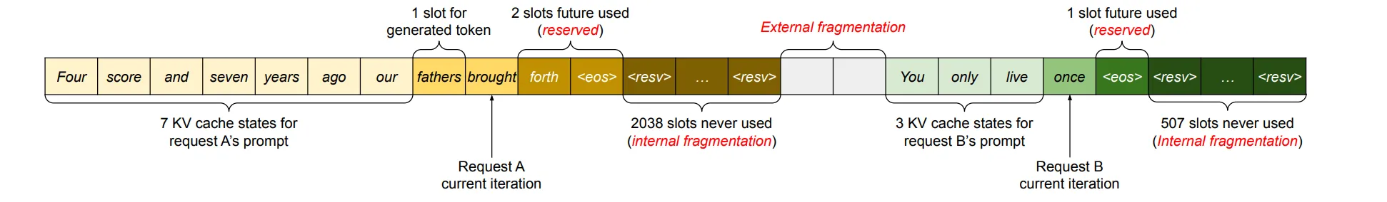
In the figure, 2048 slots are filled with one prompt of 7 words = “four, score, and, seven, years, ago, our.” The next four generated words are filled in the next slots = “fathers, brought, forth, <eos>”. It means that 2038 slots are still reserved but never used. This situation created internal fragmentation in the memory.

Each inference step generates key-value (KV) pairs that must be cached when using attention. The KV cache is typically allocated in memory in contiguous chunks or blocks (pages). After sequence generation is completed and memory pages are freed, the freed pages may not be contiguous. Subsequent sequences might need memory sizes that don’t fit neatly into existing freed blocks. This leads to small free blocks scattered throughout the memory — external fragmentation.

Inspired by OS memory management, the page attention mechanism also organises the data into a logical memory block, monitored by a page table. Then it maps the proper page into physical memory. Here are the aspects:

1. Fixed-size Blocks: PagedAttention allocates fixed-size and relatively small memory blocks called “pages” to store the KV cache.
2. Shared Blocks: These fixed-size blocks can be shared across different requests.
3. On-demand Allocation: Blocks are allocated on demand as the generation progresses, eliminating the need for upfront allocation based on maximum sequence length estimates.

Illustration for paging in LLM. Image by the author

Illustration for paging in LLM for multi request with sharing blocks. Image by the author

Raddix tree KV cache

In computer science, a radix tree (also radix trie or compact prefix tree or compressed trie) is a data structure that represents a space-optimized trie (prefix tree) in which each node that is the only child is merged with its parent. –  DBPedia

Raddix tree KV cache is a technique that enables efficient reuse of the key-value (KV) cache across different inference requests, particularly in scenarios where multiple requests share a common prefix. Organising the KV cache in the structure of a Raddix tree provides an efficient way to recall the KV cache data and easily share it among requests. In the example below, three requests shared the same prefix “ABC”, which was stored in the parent node. Then, three leaves are present for the last word in each request. Remember that running a tree costs O(nlogn), smaller than O(n²) in attention.

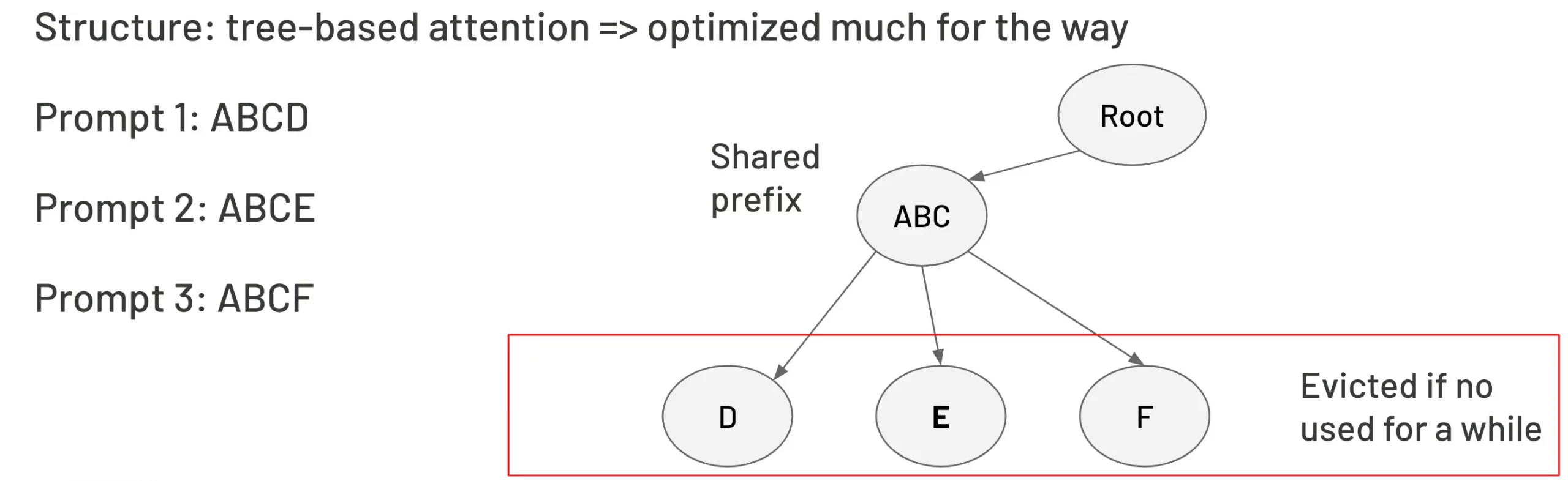
An example for Raddix tree KV cache

Compressed attention

Multi-head attention is the core of Transformer models, the backbone of LLMS. Each head looks at the text from a different point of view. One might look at how subjects and verbs relate to each other, another might look at words, and a third might look at sentence structure. This multi-head method helps us understand the model better, but it also means that each head needs its own set of KV pairs. So, when working with real-time text or longer situations, these separate Keys and Values become very large, which requires a lot of memory.

Group Query Attention (GQA) allowed Key and Value pairs to be shared among queries which reduces the number of Key and Value pairs needed to compute attention. Multi Query Attention (MQA) is the most saver while only one pair of Key and Value is used for several queries.

multi-head attention, multi-query attention, group-query attention

Deep Seek, a Chinese AI start-up, erased 1 trillion dollars early this year after releasing their chatbot. Their product works fast, effectively, and is open-source. People spread rumours about their success because of their data analysis work on the data generated by Chatgpt. However, reading their technical report gave me a vision beyond just the data extraction action. Deep Seek introduces Flash Multi Latent Attention (Flash MLA), which allows their AI scientists to train models much faster. Instead of saving the full level of K or V, they are down-projected into a latent vector with a smaller dimension by low-rank compression, resulting in the smaller cached part. Afterwards, up-projected whenever calculating the Attention. Interestingly, the up-projected matrix weight is “folded” with the matrix weight in queries, making the attention work even faster.

multi-head latent attention illustration. Image by the author

Theme 2: Query-sparsity attention

QUEST: Query-Aware Sparsity for Efficient Long-Context LLM Inference

From the paper QUEST: Query-Aware Sparsity for Efficient Long-Context LLM Inference by MIT researchers, we know that high sparsity is often present in the Transformer layers in the inference process, specifically, in the attention computation. This means not all the neural nodes in the big networks are activated during the inference time. Leveraging this idea in the pruning mechanism, we observed an effective way to run big models in the past. The below figure shows a statistic of sparsity in layers in a transformer model. Unfortunately, layers after the 3rd one are often sparse; in the worst case, some layers are 100% sparse (layer 10th, for example). This face equals that we multiply by 0 several times when running a large language model, which creates zero values.

The reason why this happens is simply because not every word contributes to the context.

For example, we have a prompt for run: “A is B. C is D. A is”. You guess, the next should be “B”, right? It’s correct. This means that only the most critical token is needed, and it depends strongly on the queries. That‘s why we call query-aware sparsity.

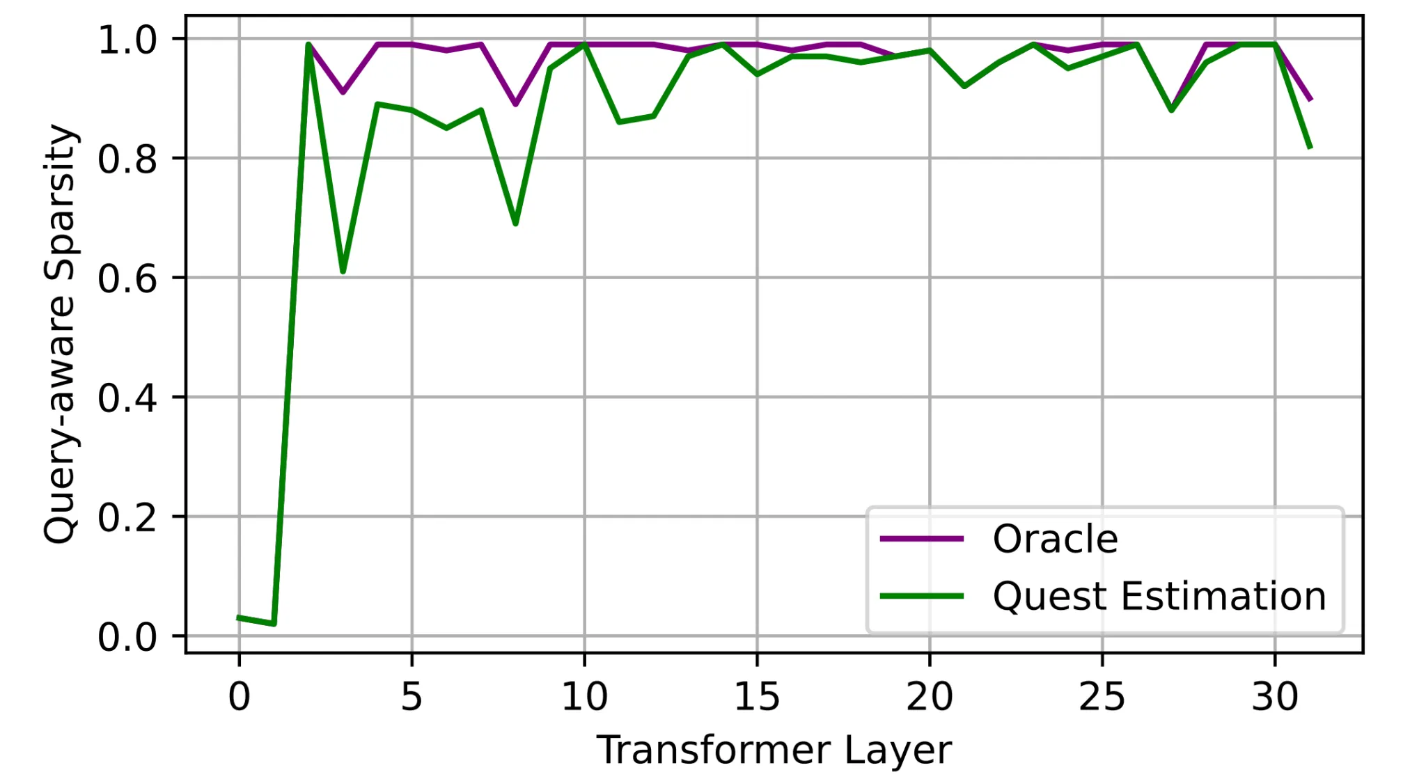
Sparsity estimation in inference of a transformer model. Image source

Understanding this trait, the strategy of QUEST is to find the block data that is most critical for the attention calculation. QUEST will discover the top K blocks of data. The algorithm is straightforward. Let’s see the below figure.

How QUEST get top k blocks to calculate attention

First, for each data block, QUEST finds the minimum and maximum keys along with the channel-wise values. Then, the query produces the max and min keys element-wise. This trick reduces the number of computations needed, and even though the sign of the query, the product action often gives the maximum value. If the query sign is negative, multiplying by the minimum value must provide the maximum output and vice versa. After conquering the maximum value of each block, QUEST selects only the top K of critically relevant KV blocks to the query. By this pipeline, our computation is reduced significantly.

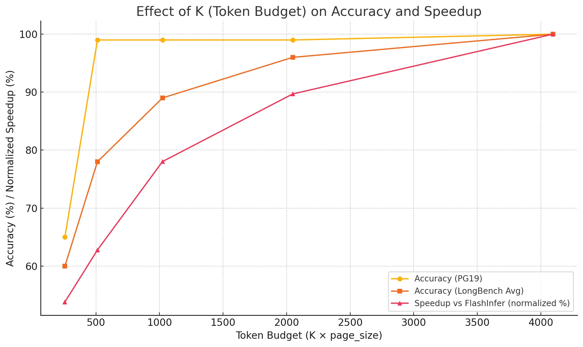
The last question we must answer is selecting the correct K value to avoid reducing the model’s performance. K is a hyperparameter that needs to be experimented with to find. In the paper, the authors suggest selecting K = 4096 to keep the performance of models nearly 100%.

Here is their data with K = 4096.

• Accuracy on PG19 (a textbook dataset) ≈ 100% of full attention
• Accuracy on passkey retrieval ≈ 100%
• Accuracy on LongBench tasks ≈ is equal to full cache on most datasets

Theme 3: Speculative decoding

Speculative decoding is essential in speeding up large language model (LLM) inference, mentioned by Andrej Karpathy and first introduced by Google in 2022.

Here’s the core idea simply:

Instead of using only the big, slow, accurate model to generate words (called the target model), we can first use a small, fast, less accurate model (often called a draft model) to “speculate” multiple following tokens quickly. Then, the big model is used to verify the guessed tokens. If the big model agrees with the small model’s guesses, you accept them all simultaneously (saving computation). If not, we fall back (redo) from the point of disagreement. Please see the illustration below.

The draft model could be Ngrams, model 1B, up to the 3B model. The target model could be billions or trillions of parameters.

Image soucre: the Internet

Using two models could be memory-consuming, and repeating the generation process also costs a lot of time. The key behind the scenes is that this technique is so practical that even big models like Gemini implemented it (the image below). The fact is that the draft model often generates tokens so correctly that the target does not need to fix the result. This is because in real life, we usually see the common words like “yes, this, is, and so on”, which are easy to guess by even small language models. Then, instead of autoregressive decoding tokens by tokens, all the generated tokens from the draft model are verified by the big one in parallel. That saves a lot of time.

In this first part, we looked at how architectural improvements like compressed attention, query-aware sparsity, and speculative decoding might help address key LLM serving concerns including KV cache expansion, memory bottlenecks, and decoding inefficiencies. These methodologies lay the groundwork for efficient inference at the algorithm level, paving the way for even larger-scale implementations.
In the next part, we’ll shift gears and look at system-level and deployment-oriented solutions, where infrastructure considerations, scheduling methods, and hardware-aware tricks can result in substantial performance benefits in real-world applications.